
Using geometry to identify overlapping attribute ranges.
Two of the most interesting concepts I have encountered in my career both relate to the issue of describing the physical connectivity of a linear network through attributes rather than geometry. Specifically, I am referring to (1) Linear Referencing Systems and their corresponding Measures widely used in the Transportation Industry, and (2) road network address ranges used in local governments and 9-1-1 systems nationwide. While the following logic can be applied to both of these areas, we are going to investigate this using road centerline address ranges.
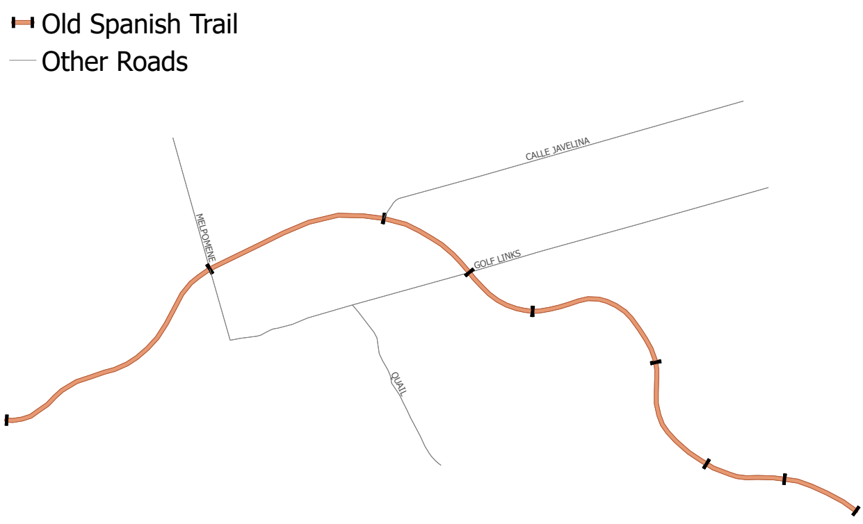
Imagining a road from a top-down perspective, we can easily visualize a 2-dimension line that may twist, turn and curve along its route. In the following image, we see the road Old Spanish Trail in Pima County represented as an orange line. The road has been split into segments where it intersects other roads and these intersections have been represented as black bars cutting perpendicular through the Old Spanish Trail.
Expanding further on this, we can visualize the address range attributes as colored labels, showing FROM address ranges in green, and TO address ranges in red.
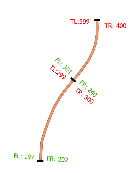
Here we have two segments of Old Spanish, with each segment’s left and right address ranges labeled.
Segment 1
- Left range: 197 -> 299
- Right range: 202 -> 300
Segment 2
- Left range: 301 -> 399
- Right range: 240-> 400
In the above scenario, we visualize an Address Range Overlap. Specifically, the address range of the right side of segment two ends at 300, but the following segment’s right address range begins at 240. This would mean that the addresses along Old Spanish Trail whose house numbers fall into the range 240-300 technically exist on both segment 1, and segment 2.
Not only is this inconceivable, but could you imagine the headache emergency services personnel would get trying to determine where to go when someone at 275 Old Spanish Trail called 9-1-1? Is their house along segment 1? Is there a house along segment two? Are there multiple houses with the address 275 Old Spanish Trail
In this case, it’s easy to see the discrepancy when we look at 2 records. But what if we had to look at 10,000 records? or 2,000,000 records? The process of manual identification quickly becomes unmanageable. Sure, this problem could be solved through complex SQL queries combining Lag/Lead functions with a Window function, altering the sorting order, and looking for where one record overlaps another. That process would certainly be able to identify a record overlapping its nearest neighbor in the sort order, but what would you sort on? from measure, or to measure? and would the process be able to identify if one record overlapped with many records, potentially 20+ records away in the lag/lead window?
Let's explore an alternative!
In both the case of the From/To Measure values in Linear Referencing Systems and the From/To address ranges in road centerline networks, these attribute values are meant to model the real world characteristics. However, these values are:
(1) Agnostic of their features physical geometry in the sense that they only represent distance along an axis parallel to the linear feature, completely ignoring any bends twists, or turns along the feature
and
(2) discrete in the sense that they exist in their own location and should not contain overlaps.
*Note – In the case of LRS Event Layers, some layers may contain overlapping events, but many layers and the route network itself should not. For instance, You probably should not have overlapping # of Through Lanes, because how could the roadway have both 3 through lanes and 5 through lanes in the same location?
Given the two above assumptions, we can translate the curves of our roadway to a linear graph, and plot the address ranges of the right side of the roadway along a single axis of a graph to visualize this overlap as seen below.
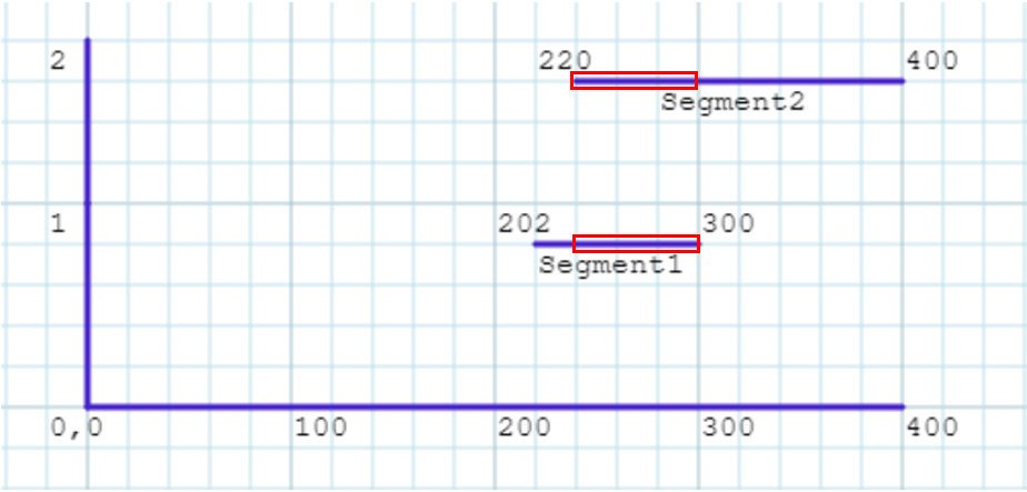
Above, we have plotted segment 1 as a straight line along one dimension, keepings its y-value constant. Its coordinates are (202,1), and (300,1). Segment 2 has been plotted similarly, except kept constant along a y-axis value of 2. Its coordinate values are (220,2) and (400,2). The overlapping ranges have been highlighted in red boxes. Again, we are only interested in comparing ranges, not the true geometry of the feature.
Now, imagine that instead of plotting the lines on a paper graph, we (1) used the measures to create physical geometry in a simple coordinate system using a basic cartesian plane and (2) kept the y axis value for both lines constant so that both lines drew along the same axis.
The result is two straight line geometries that we can run an intersect function on to identify if, and where, the lines intersect. This can be scaled up nearly infinitely and is limited only by the performance of the GIS software engine and your hardware. Because this defined coordinate space is small, and requires very little math for the spatial engines, this process is very performant as well.
Let's see what this process looks like in Safe Software's FME
The entirety of the process, in its simplest forms, is comprised of just 13 steps that applied to each the right side and left side address ranges. Some of the 13 steps are simple logic tests, or attribute configuration steps meaning the bulks of the actual process to identify these overlaps happens in around 10 individuals steps. First, let’s walk through the process together and at the end I’ll provide a sample workspace for you to run. Below is a screenshot of the entire workspace, identifying overlaps in both the left and right address ranges. Each of the individual block below is called a Transformer.
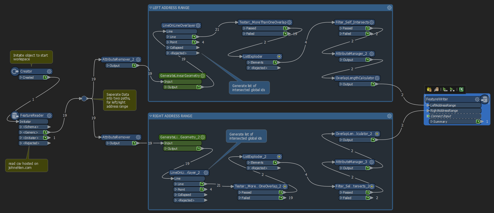
While the above screenshot shows both the left and right address ranges, I will only be walking through the left address range workflow because the process is identical for the right side, with just the relevant field names substituted for right instead of left.
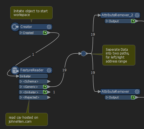
To begin the workspace, we use a Creator Transformer to initiate an empty object.
This empty object is then passed to our FeatureReader Transformer as the initiator, and the FeatureReader reads a CSV dataset from a web URL
The incoming data is then duplicated into two streams, one for left address ranges, and one for right address ranges. this is done by using a Junction and attaching the output twice
The records are then supplied to an AttributeRemover, which removes the unneeded attributes. (Left address range process doesn’t need right ranges, vice versa.)
The next step of the process actually involves a custom transformer embedded within the workspace. This custom transformer allows us to apply the same operations to different sets of data and is reusable. If you’re familiar with programming, you can think of the custom transformer as a function. It takes an input, does something, and returns the results.
Below (left), you can see a green box titled “GenerateLinearGeometry”. This is our custom transformer.
Below (right), you can see the contents of our custom transformer including the data input and output ports (click to enlarge).
Let’s investigate what this custom transformer is doing.
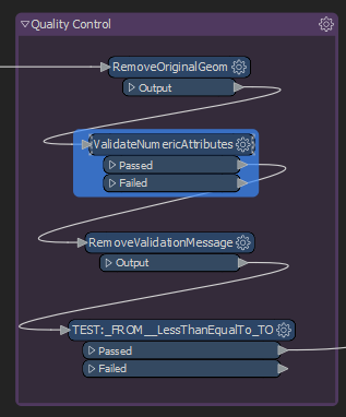
Inside the custom transformer, the first we do is run a series of quality control steps. The prevents issues later on when we try and insert new vertices.
- Remove the original Geometry of the incoming data(GeometryRemover)
- Validate measure attributes are numeric (AttributeValidator).
- Next, we strip the validation message as it’s not needed (AttributeRemover).
- Finally, we test to ensure our from value is less than our to value. (Tester)
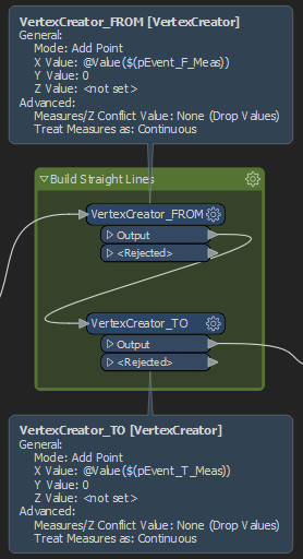
Now that we’ve stripped the original geometry and validated the quality of our data attributes, we can build the new straight-line geometry. This is done in two steps:
1. For each incoming feature, we add a new vertex using the VertexCreator Transformer. We assign the X-Coord of the vertex to be the from measure, and we kept the Y-Value of the coordinate constant, with a value of zero.
2. We repeat the process for the second vertex, but this time using the to measure as the X-Coord, and still keeping the Y-Coord constant with a value of zero.
By doing this, we plot each individual line segment in the same coordinate space along the same y-axis, meaning we have linear segments spanning a horizontal distance just as shown before in the graph paper screenshot. However, instead of our lines being drawn in two different planes (Y-value 1, Y-value 2), they are drawn along the same plane (Y-value 0) and thus can be geometrically intersected.
* A note about the VertexCreator Transformer – The reason the process works, the process only adds vertices to the record currently being processed. Additionally, the vertex will atomically shift the geometry of the resulting feature based on the following criteria:
1 vertex on feature will results in point geometry
2 vertices on feature will result in linear geometry
>2 Vertices on feature AND firstVertex = lastVertex results in polygon geometry
Now we’ve reached the end of the custom transformer, or function, and the result is new linear geometry built along a single axis. From here, we can continue the process to identify overlapping ranges.
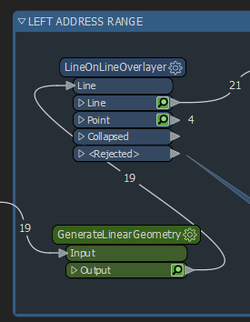
After we have generated the linear geometry, we then need to intersect it with itself, we do this the LineOnLineOverlayer.
Because our address ranges exist on different streets, and in different locations (cities, zip codes, states, etc) it’s important to group these so we don’t identify overlaps that are not related to each other. By grouping these items with their related segments with the group processing option of this transformer, we ensure that we only detect real overlaps.
In the dialog options, we also choose to generate a list attribute, adding the FromRange, ToRange, and Unique ID Attributes. We will use this list shortly.
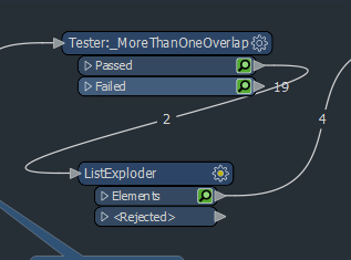
Next, we use a Tester Transformer with a simple test: Where we have more than 1 overlap. We check for more than one overlap because in FME an object will intersect itself, so it should always have one overlap.
Next, we use the ListExploder Transformer to deaggregate the list items that the LineOnLineOverlayer generated. The result is a table that shows us each overlap as seen below
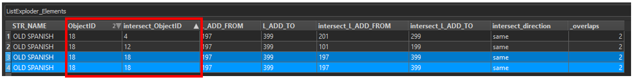
However, our table isn’t quite correct yet. If we look at the the two records selected in blue, and we look at the two columns outlined in red, we can see we are reporting self intersects. This is because, as mentioned previously, geometry will always self intersect in FME. Previously, we discarded records if they only had one intersect (self overlap), now we need to discard the self intersects from the rest of the records with >1 overlap.
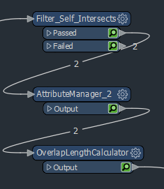
To do this, we use a simple Tester to see if the object id of the original feature is equal to the object id of the intersected feature. If they are the same, we just disregard it.
In the AttributeManager Transformer, minor formatting is applied and some unneeded columns are removed.
Next, we finally calculate the length of the overlap by using
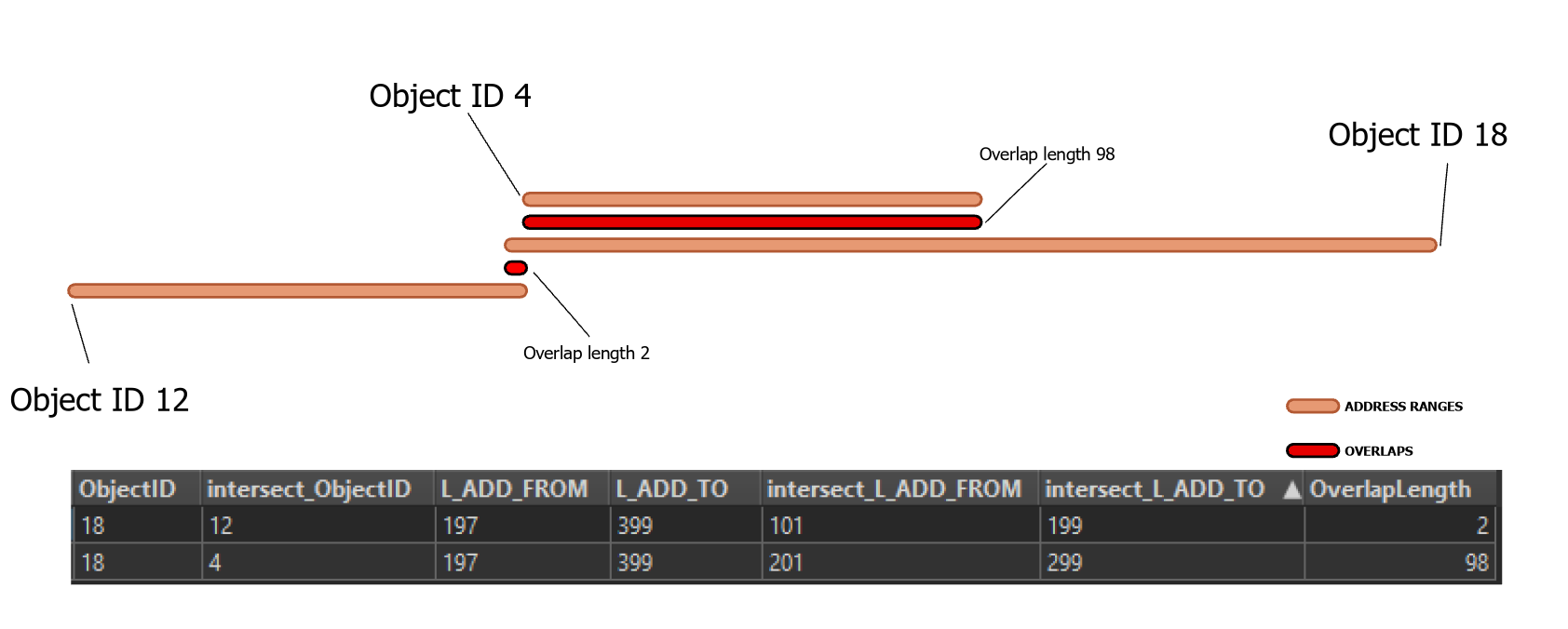
Below, I’ve visualized the results using a straight-line diagram. The address ranges themselves are represented in orange, while the range where the overlap is represented in red.
We can see OBJECTID 18 is the culprit and covers the enter length of OBJECTID 4, as well as overlaps into the range of OBJECTID 12 as well.
You sir, are amazing. Thank you for sharing this with me!